Exercise_10: The Solar System
2016-11-27 本文已影响0人
Damonphysics
We begin with the simplest situation,a sun and a single planet,and investigate a few of the properties of this model solar system.
 solar system.gif
 solar system.gif
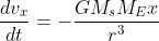
According to Newton's law of gravitation the magnitude of the force is given by
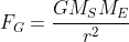
and we can obtain that:
 Earth Orbiting the Sun
code1,as follows:
#coding:utf-8
import pylab as pl
import numpy as np
import math
from mpl_toolkits.mplot3d import Axes3D
import matplotlib.pyplot as plt
from matplotlib import animation

class circle():
    def __init__(self,x0=1,y0=0,t0=0,vx0=0,vy0=2*math.pi,dt0=0.001,total_time=10):
        self.x=[x0]
        self.y=[y0]
        self.vx=[vx0]
        self.vy=[vy0]
        self.R=x0**2+y0**2
        self.t=[t0]
        self.dt=dt0
        self.T=total_time
    def run(self):
        for i in range(int(self.T/self.dt)):
            vx=self.vx[-1]-(4*math.pi**2*self.x[-1]/self.R**2)*self.dt
            vy=self.vy[-1]-(4*math.pi**2*self.y[-1]/self.R**2)*self.dt
            self.vx.append(vx)
            self.vy.append(vy)
            self.x.append(self.vx[-1] * self.dt + self.x[-1])
            self.y.append(self.vy[-1] * self.dt + self.y[-1])
    def show(self):
        pl.plot(self.x, self.y, '-', label='tra')
        pl.xlabel('x(AU)')
        pl.ylabel('y(AU)')
        pl.title('Earth orbiting the Sun')
        pl.xlim(-1.2,1.2)
        pl.ylim(-1.2,1.2)
        pl.axis('equal')
        pl.show()
a=circle()
a.run()
a.show()
we can use the animation of matplotlib to gain the cartoon,
add follow codes:
 def drawtrajectory(self):
        fig=plt.figure()
        ax = plt.axes(title=('Earth orbiting the Sun'),
                      aspect='equal', autoscale_on=False,
                      xlim=(-1.1, 1.1), ylim=(-1.1, 1.1),
                      xlabel=('x'),ylabel=('y'))
        line=ax.plot([],[],'b')
        point=ax.plot([],[],'ro',markersize=10)
        images=[]
        def init():
            line=ax.plot([],[],'b',markersize=8)
            point=ax.plot([],[],'ro',markersize=10)
            return line,point
        def anmi(i):
            ax.clear()
            line=ax.plot(self.x[0:10*i],self.y[0:10*i],'b',markersize=8)
            point=ax.plot(self.x[10*i-1:10*i],self.y[10*i-1:10*i],'ro',markersize=10)
            return line,point
        anmi=animation.FuncAnimation(fig,anmi,init_func=init,frames=10000,interval=1,
                                     blit=False,repeat=False)
we get follow gif
 Earth Orbiting the Sun
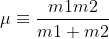
If we consider the reduced mass
The orbital trajectory for a body of reduced mass is given in polar coordinates by
+\frac{1}{r}=-\frac{\mu r2}{L2} F(r))
consider
 Beta=3.0 t=0.3yr v=1.7pi.png
 Beta=2.5,t=1.5yr,v=1.7pi.png
 Beta=2.3,t=10yr,v=1.7pi.png
code
#coding:utf-8
import pylab as pl
import numpy as np
import math
from mpl_toolkits.mplot3d import Axes3D
import matplotlib.pyplot as plt
from matplotlib import animation

class circle():
    def __init__(self,x0=1,y0=0,t0=0,vx0=0,vy0=1.7*math.pi,dt0=0.001,Beta=2.3,total_time=10):
        self.x=[x0]
        self.y=[y0]
        self.vx=[vx0]
        self.vy=[vy0]
        self.t=[t0]
        self.dt=dt0
        self.T=total_time
        self.beta=Beta
    def run(self):
        for i in range(int(self.T/self.dt)):
            R=(self.x[-1]**2+self.y[-1]**2)**0.5
            vx=self.vx[-1]-(4*math.pi**2*self.x[-1]/R**(self.beta+1))*self.dt
            vy=self.vy[-1]-(4*math.pi**2*self.y[-1]/R**(self.beta+1))*self.dt
            self.vx.append(vx)
            self.vy.append(vy)
            self.x.append(self.vx[-1] * self.dt + self.x[-1])
            self.y.append(self.vy[-1] * self.dt + self.y[-1])
    def show(self):
        pl.plot(self.x, self.y, '-', label='tra')
        pl.xlabel('x(AU)')
        pl.ylabel('y(AU)')
        pl.title('Earth orbiting the Sun')
        pl.xlim(-1,1)
        pl.ylim(-1,1)
        pl.axis('equal')
        pl.show()
    def drawtrajectory(self):
        fig=plt.figure()
        ax = plt.axes(title=('Earth orbiting the Sun '),
                      aspect='equal', autoscale_on=False,
                      xlim=(-1.1, 1.1), ylim=(-1.1, 1.1),
                      xlabel=('x'),ylabel=('y'))
        line=ax.plot([],[],'b')
        point=ax.plot([],[],'ro',markersize=10)
        images=[]
        def init():
            line=ax.plot([],[],'b',markersize=8)
            point=ax.plot([],[],'ro',markersize=10)
            return line,point
        def anmi(i):
            ax.clear()
            line=ax.plot(self.x[0:10*i],self.y[0:10*i],'b',markersize=8)
            point=ax.plot(self.x[10*i-1:10*i],self.y[10*i-1:10*i],'ro',markersize=10)
            return line,point
        anmi=animation.FuncAnimation(fig,anmi,init_func=init,frames=100000,interval=1,
                                     blit=False,repeat=False)
        plt.show()


a=circle()
a.run()
a.show()
#a.drawtrajectory()
then we get the animation
 Beta=3.0,v=2.0pi,t=200yr
for the problem 4.8, I use the follow code to calculate
import pylab as pl
import numpy as np
import math
class circle():
    def __init__(self,x0=0.72,y0=0,t0=0,vx0=0,dt0=0.001,Beta=2.0,total_time=10,e0=0.007):
        self.x=[x0]
        self.y=[y0]
        self.vx=[vx0]
        self.vy=[]
        self.t=[t0]
        self.dt=dt0
        self.T=total_time
        self.beta=Beta
        self.e=e0

    def run(self):
        vy0=2*math.pi*(1-self.e)/math.sqrt(1+self.e)
        self.vy.append(vy0)
        for i in range(int(self.T/self.dt)):
            R=(self.x[-1]**2+self.y[-1]**2)**0.5
            vx=self.vx[-1]-(4*math.pi**2*self.x[-1]/R**(self.beta+1))*self.dt
            vy=self.vy[-1]-(4*math.pi**2*self.y[-1]/R**(self.beta+1))*self.dt
            self.vx.append(vx)
            self.vy.append(vy)
            self.x.append(self.vx[-1] * self.dt + self.x[-1])
            self.y.append(self.vy[-1] * self.dt + self.y[-1])
            self.t.append(self.t[-1]+self.dt)
            if(self.y[-1]<0):
                a=(self.x[0]-self.x[-1])/2
                T=2*self.t[-1]
                k=T**2/a**3
                break
        print(k)
a=circle()
a.run()


